
Who do we target for Donations
- We have a dataset of people we approached for doners for our Election campaign
- We have their education, job, income, ethnicity
- We know high income earners are better to approach for political donations
Let's build a classifier that predicts income levels based on a person's attributes.
Those will be the persons we appraoch first for political donations
Feature explanation:
age: continuous. workclass: Private, Self-emp-not-inc, Self-emp-inc, Federal-gov, Local-gov, State-gov, Without-pay, Never-worked.
workclass: categorical data; different types of work class
fnlwgt: Final weight; Its a weight assigned by the US census bureau to each row. The literal meaning is that you will need to replicate each row, final weight times to get the full data. And it would be somewhat 6.1 billion rows in it. Dont be shocked by the size, its an accumulated data over decades.
education: Bachelors, Some-college, 11th, HS-grad, Prof-school, Assoc-acdm, Assoc-voc, 9th, 7th-8th, 12th, Masters, 1st-4th, 10th, Doctorate, 5th-6th, Preschool.
education-num: continuous.
marital-status: Married-civ-spouse, Divorced, Never-married, Separated, Widowed, Married-spouse-absent, married-F-spouse.
occupation: Tech-support, Craft-repair, Other-service, Sales, Exec-managerial, Prof-specialty, Handlers-cleaners, Machine-op-inspect, Adm-clerical, Farming-fishing, Transport-moving, Priv-house-serv, Protective-serv, Armed-Forces.
relationship: Wife, Own-child, Husband, Not-in-family, Other-relative, Unmarried.
race: Black, White, Asian-Pac-Islander, Amer-Indian-Eskimo, Other.
sex: Female, Male.
capital-gain: continuous.
capital-loss: continuous.
hours-per-week: continuous.
native-country: United-States, Cambodia, England, Puerto-Rico, Canada, Germany, Outlying-US(Guam-USVI-etc), India, Japan, Greece, South, China, Cuba, Iran, Honduras, Philippines, Italy, Poland, Jamaica, Vietnam, Mexico, Portugal, Ireland, France, Dominican-Republic, Laos, Ecuador, Taiwan, Haiti, Columbia, Hungary, Guatemala, Nicaragua, Scotland, Thailand, Yugoslavia, El-Salvador, Trinadad&Tobago, Peru, Hong, Holand-Netherlands.
Income: Whether a person's income is more than $50,000 or not. This is our dependent variable.
We are going to create a classification model using Decision Tree, Random Forest, and XGBoost using Python. At the end we will compare the results to zero down on the best model.
    import numpy as np
    import pandas as pd
    import os
    from matplotlib import pyplot as plt
    pd.options.mode.chained_assignment = None  # removes warning messages

    os.chdir("C:\\Users\\ASUS")
    census = pd.read_csv("adult.csv")
    census.head()
| age | workclass | fnlwgt | education | education-num | marital-status | occupation | relationship | race | sex | capital-gain | capital-loss | hours-per-week | native-country | Income | |
|---|---|---|---|---|---|---|---|---|---|---|---|---|---|---|---|
| 0 | 50 | Self-emp-not-inc | 83311 | Bachelors | 13 | Married-civ-spouse | Exec-managerial | Husband | White | Male | 0 | 0 | 13 | United-States | <=50K |
| 1 | 38 | Private | 215646 | HS-grad | 9 | Divorced | Handlers-cleaners | Not-in-family | White | Male | 0 | 0 | 40 | United-States | <=50K |
| 2 | 53 | Private | 234721 | 11th | 7 | Married-civ-spouse | Handlers-cleaners | Husband | Black | Male | 0 | 0 | 40 | United-States | <=50K |
| 3 | 28 | Private | 338409 | Bachelors | 13 | Married-civ-spouse | Prof-specialty | Wife | Black | Female | 0 | 0 | 40 | Cuba | <=50K |
| 4 | 37 | Private | 284582 | Masters | 14 | Married-civ-spouse | Exec-managerial | Wife | White | Female | 0 | 0 | 40 | United-States | <=50K |
Observation: Income is given as an object (character). We will modify this column as 1 (<=50K), else 0
#Unique values of Income variable
                census.Income.unique()
array([' <=50K', ' >50K'], dtype=object)
#Frequency distribution of Income variable
                census.Income.value_counts()
 <=50K    24719
                 >50K      7841
                Name: Income, dtype: int64
census["Income"] = np.where(census["Income"] == ' <=50K',0,1 )
#Frequency distribution of Income variable
                census.Income.value_counts()
0    24719
                1     7841
                Name: Income, dtype: int64
Observation: Income variable has been correctly modified as 1 and 0
census.head(2)
| age | workclass | fnlwgt | education | education-num | marital-status | occupation | relationship | race | sex | capital-gain | capital-loss | hours-per-week | native-country | Income | |
|---|---|---|---|---|---|---|---|---|---|---|---|---|---|---|---|
| 0 | 50 | Self-emp-not-inc | 83311 | Bachelors | 13 | Married-civ-spouse | Exec-managerial | Husband | White | Male | 0 | 0 | 13 | United-States | 0 |
| 1 | 38 | Private | 215646 | HS-grad | 9 | Divorced | Handlers-cleaners | Not-in-family | White | Male | 0 | 0 | 40 | United-States | 0 |
Missing value Treatment
# number of missing values by variables
                census.isnull().sum()
age               0
                workclass         0
                fnlwgt            0
                education         0
                education-num     0
                marital-status    0
                occupation        0
                relationship      0
                race              0
                sex               0
                capital-gain      0
                capital-loss      0
                hours-per-week    0
                native-country    0
                Income            0
                dtype: int64
Observation: There are no missing values in the data
Exploratory Data Analysis (EDA)
#segregating the numeric and categorical variables
                dataset_categorical = census.select_dtypes(exclude = "number")
                dataset_numeric = census.select_dtypes(include = "number")
#create the dummy variables
                #dataset_categorical= pd.get_dummies(data = dataset_categorical, drop_first = True)
                dataset_categorical.head(2)
| workclass | education | marital-status | occupation | relationship | race | sex | native-country | |
|---|---|---|---|---|---|---|---|---|
| 0 | Self-emp-not-inc | Bachelors | Married-civ-spouse | Exec-managerial | Husband | White | Male | United-States |
| 1 | Private | HS-grad | Divorced | Handlers-cleaners | Not-in-family | White | Male | United-States |
dataset_categorical.describe(include='object')
| workclass | education | marital-status | occupation | relationship | race | sex | native-country | |
|---|---|---|---|---|---|---|---|---|
| count | 32560 | 32560 | 32560 | 32560 | 32560 | 32560 | 32560 | 32560 |
| unique | 9 | 16 | 7 | 15 | 6 | 5 | 2 | 42 |
| top | Private | HS-grad | Married-civ-spouse | Prof-specialty | Husband | White | Male | United-States |
| freq | 22696 | 10501 | 14976 | 4140 | 13193 | 27815 | 21789 | 29169 |
We can see that there are leading and/or trailing spaces
dataset_categorical["native-country"].unique()
array([' United-States', ' Cuba', ' Jamaica', ' India', ' ?', ' Mexico',
                       ' South', ' Puerto-Rico', ' Honduras', ' England', ' Canada',
                       ' Germany', ' Iran', ' Philippines', ' Italy', ' Poland',
                       ' Columbia', ' Cambodia', ' Thailand', ' Ecuador', ' Laos',
                       ' Taiwan', ' Haiti', ' Portugal', ' Dominican-Republic',
                       ' El-Salvador', ' France', ' Guatemala', ' China', ' Japan',
                       ' Yugoslavia', ' Peru', ' Outlying-US(Guam-USVI-etc)', ' Scotland',
                       ' Trinadad&Tobago', ' Greece', ' Nicaragua', ' Vietnam', ' Hong',
                       ' Ireland', ' Hungary', ' Holand-Netherlands'], dtype=object)
We will use the following code to remove all leading and trailing spaces from all variables
dataset_categorical= dataset_categorical.apply(lambda x: x.str.strip() if x.dtype == "object" else x)
We can see that there are instances where we have question marks ("?"). We will replace them by their respective mode
dataset_categorical["native-country"].value_counts()
United-States                 29169
                Mexico                          643
                ?                               583
                Philippines                     198
                Germany                         137
                Canada                          121
                Puerto-Rico                     114
                El-Salvador                     106
                India                           100
                Cuba                             95
                England                          90
                Jamaica                          81
                South                            80
                China                            75
                Italy                            73
                Dominican-Republic               70
                Vietnam                          67
                Guatemala                        64
                Japan                            62
                Poland                           60
                Columbia                         59
                Taiwan                           51
                Haiti                            44
                Iran                             43
                Portugal                         37
                Nicaragua                        34
                Peru                             31
                Greece                           29
                France                           29
                Ecuador                          28
                Ireland                          24
                Hong                             20
                Trinadad&Tobago                  19
                Cambodia                         19
                Laos                             18
                Thailand                         18
                Yugoslavia                       16
                Outlying-US(Guam-USVI-etc)       14
                Hungary                          13
                Honduras                         13
                Scotland                         12
                Holand-Netherlands                1
                Name: native-country, dtype: int64
#We will replace the ? (which seems to be missing value) with mode, i.e. United-States
                dataset_categorical["native-country"]= dataset_categorical["native-country"].str.replace("?","United-States")
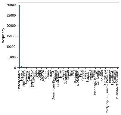
Observations: Distribution of native-country shows United-States alone is there for majority of the rows for this variable. Hence, we will not count rest of the countries separately, but club them together as others. Then we will code United-States as 1 and others 0 to create a dummy variable
dataset_categorical["native-country"].value_counts().plot(kind='bar', ylabel='frequency')
                plt.show()
dataset_categorical["native-country"] = np.where(dataset_categorical["native-country"] == "United-States",1,0 )
Native-country has been converted into a dummy variable
dataset_categorical["native-country"].value_counts()
1    29752
                0     2808
                Name: native-country, dtype: int64
Now we will do the same treatment with other categorical variables
dataset_categorical["workclass"].value_counts()
Private             22696
                Self-emp-not-inc     2541
                Local-gov            2093
                ?                    1836
                State-gov            1297
                Self-emp-inc         1116
                Federal-gov           960
                Without-pay            14
                Never-worked            7
                Name: workclass, dtype: int64
#We will replace the ? (which seems to be missing value) with mode, i.e. Private
                dataset_categorical["workclass"]= dataset_categorical["workclass"].str.replace("?","Private")
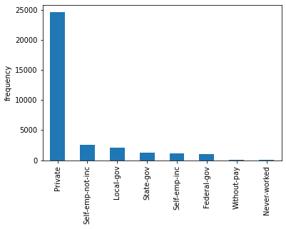
dataset_categorical["workclass"].value_counts().plot(kind='bar', ylabel='frequency')
                plt.show()
dataset_categorical["workclass"] = np.where(dataset_categorical["workclass"] == "Private",1,0 )
dataset_categorical["workclass"].value_counts()
1    24532
                0     8028
                Name: workclass, dtype: int64
dataset_categorical["occupation"].value_counts()
Prof-specialty       4140
                Craft-repair         4099
                Exec-managerial      4066
                Adm-clerical         3769
                Sales                3650
                Other-service        3295
                Machine-op-inspct    2002
                ?                    1843
                Transport-moving     1597
                Handlers-cleaners    1370
                Farming-fishing       994
                Tech-support          928
                Protective-serv       649
                Priv-house-serv       149
                Armed-Forces            9
                Name: occupation, dtype: int64
#We will replace the ? (which seems to be missing value) with mode, i.e. Prof-specialty
                dataset_categorical["occupation"]= dataset_categorical["occupation"].str.replace("?","Prof-specialty")
dataset_categorical["occupation"].value_counts().plot(kind='bar', ylabel='frequency')
                plt.show()
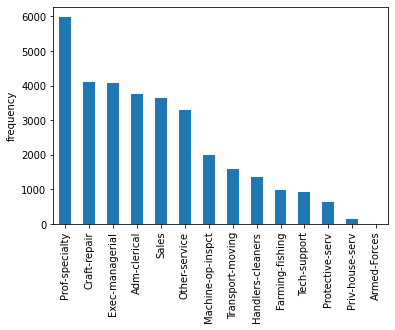
We will club the last 5 categories as "others" where the frequencies are less than 1000
dataset_categorical["occupation"] = np.where(dataset_categorical["occupation"].isin(["Farming-fishing",
                "Tech-support","Protective-serv","Priv-house-serv","Armed-Forces"]),"others",dataset_categorical["occupation"])
dataset_categorical.head(2)
| workclass | education | marital-status | occupation | relationship | race | sex | native-country | |
|---|---|---|---|---|---|---|---|---|
| 0 | 0 | Bachelors | Married-civ-spouse | Exec-managerial | Husband | White | Male | 1 |
| 1 | 1 | HS-grad | Divorced | Handlers-cleaners | Not-in-family | White | Male | 1 |
Dummy Variable creation
dataset_categorical=pd.get_dummies(data=dataset_categorical,columns=['education', 'marital-status',
                "occupation","relationship","race","sex"],drop_first=True)
All the dummy variables have been properly created
dataset_categorical.head(2)
| workclass | native-country | education_11th | education_12th | education_1st-4th | education_5th-6th | education_7th-8th | education_9th | education_Assoc-acdm | education_Assoc-voc | ... | relationship_Not-in-family | relationship_Other-relative | relationship_Own-child | relationship_Unmarried | relationship_Wife | race_Asian-Pac-Islander | race_Black | race_Other | race_White | sex_Male | |
|---|---|---|---|---|---|---|---|---|---|---|---|---|---|---|---|---|---|---|---|---|---|
| 0 | 0 | 1 | 0 | 0 | 0 | 0 | 0 | 0 | 0 | 0 | ... | 0 | 0 | 0 | 0 | 0 | 0 | 0 | 0 | 1 | 1 |
| 1 | 1 | 1 | 0 | 0 | 0 | 0 | 0 | 0 | 0 | 0 | ... | 1 | 0 | 0 | 0 | 0 | 0 | 0 | 0 | 1 | 1 |
2 rows × 42 columns
dataset_numeric.head(2)
| age | fnlwgt | education-num | capital-gain | capital-loss | hours-per-week | Income | |
|---|---|---|---|---|---|---|---|
| 0 | 50 | 83311 | 13 | 0 | 0 | 13 | 0 |
| 1 | 38 | 215646 | 9 | 0 | 0 | 40 | 0 |
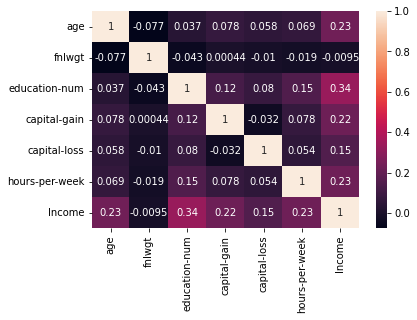
The correlations are within control. We don't find any variable with correlation of .8 or more.
import seaborn as sns
                import matplotlib.pyplot as plt
                correlation_mat = dataset_numeric.corr()
                sns.heatmap(correlation_mat, annot = True)
                plt.show()
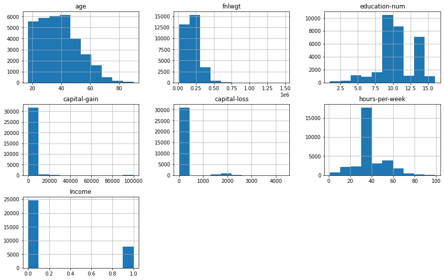
#Distribution plot
                dataset_numeric.hist(figsize=(15,30),layout=(9,3))
array([[<AxesSubplot:title={'center':'age'}>,
                        <AxesSubplot:title={'center':'fnlwgt'}>,
                        <AxesSubplot:title={'center':'education-num'}>],
                       [<AxesSubplot:title={'center':'capital-gain'}>,
                        <AxesSubplot:title={'center':'capital-loss'}>,
                        <AxesSubplot:title={'center':'hours-per-week'}>],
                       [<AxesSubplot:title={'center':'Income'}>, <AxesSubplot:>,
                        <AxesSubplot:>],
                       [<AxesSubplot:>, <AxesSubplot:>, <AxesSubplot:>],
                       [<AxesSubplot:>, <AxesSubplot:>, <AxesSubplot:>],
                       [<AxesSubplot:>, <AxesSubplot:>, <AxesSubplot:>],
                       [<AxesSubplot:>, <AxesSubplot:>, <AxesSubplot:>],
                       [<AxesSubplot:>, <AxesSubplot:>, <AxesSubplot:>],
                       [<AxesSubplot:>, <AxesSubplot:>, <AxesSubplot:>]], dtype=object)
dataset_numeric.drop("fnlwgt",axis=1,inplace=True)
                dataset_numeric.head(2)
| age | education-num | capital-gain | capital-loss | hours-per-week | Income | |
|---|---|---|---|---|---|---|
| 0 | 50 | 13 | 0 | 0 | 13 | 0 |
| 1 | 38 | 9 | 0 | 0 | 40 | 0 |
Concatenate the datasets to get the final data
#dataset_categorical = census.select_dtypes(exclude = "number")
                #dataset_numeric = census.select_dtypes(include = "number")
                data = pd.concat([dataset_categorical,dataset_numeric],axis=1)
data.head(2)
| workclass | native-country | education_11th | education_12th | education_1st-4th | education_5th-6th | education_7th-8th | education_9th | education_Assoc-acdm | education_Assoc-voc | ... | race_Black | race_Other | race_White | sex_Male | age | education-num | capital-gain | capital-loss | hours-per-week | Income | |
|---|---|---|---|---|---|---|---|---|---|---|---|---|---|---|---|---|---|---|---|---|---|
| 0 | 0 | 1 | 0 | 0 | 0 | 0 | 0 | 0 | 0 | 0 | ... | 0 | 0 | 1 | 1 | 50 | 13 | 0 | 0 | 13 | 0 |
| 1 | 1 | 1 | 0 | 0 | 0 | 0 | 0 | 0 | 0 | 0 | ... | 0 | 0 | 1 | 1 | 38 | 9 | 0 | 0 | 40 | 0 |
2 rows × 48 columns
#segregate data into dependent and independent variables

                X = data.drop("Income", axis = 1)#independent variables
                y = data["Income"]#dependent variable
Now we will split the data into training (80% of the data) and rest 20% - named test, will be kept aside for later use.
# Splitting it into training and testing (70% train & 30% test)
                from sklearn.model_selection import train_test_split
                X_train, X_test, y_train, y_test = train_test_split(X, y, test_size = 0.3, random_state = 42)
from sklearn.tree import DecisionTreeClassifier
classifier = DecisionTreeClassifier(random_state=0)
                classifier.fit(X_train, y_train)
DecisionTreeClassifier(random_state=0)
Predict the model
y_pred = classifier.predict(X_test)
Check accuracy with Classification report
from sklearn.metrics import classification_report, confusion_matrix, accuracy_score
                print(classification_report(y_test,y_pred))
              precision    recall  f1-score   support

                           0       0.87      0.89      0.88      7395
                           1       0.62      0.58      0.60      2373

                    accuracy                           0.81      9768
                   macro avg       0.75      0.73      0.74      9768
                weighted avg       0.81      0.81      0.81      9768
Collating the Report
report = classification_report(y_test,y_pred, output_dict=True)
                df = pd.DataFrame(report).transpose()
                #df
                import numpy as np
                df["model"]="Decision Tree"
                df1 = df.iloc[0:3,np.r_[0:3,4] ]
                df1
| precision | recall | f1-score | model | |
|---|---|---|---|---|
| 0 | 0.868724 | 0.886815 | 0.877677 | Decision Tree |
| 1 | 0.622803 | 0.582385 | 0.601916 | Decision Tree |
| accuracy | 0.812858 | 0.812858 | 0.812858 | Decision Tree |
from sklearn.ensemble import RandomForestClassifier
rf = RandomForestClassifier(n_estimators=1000,random_state=0)
                rf.fit(X_train, y_train)
RandomForestClassifier(n_estimators=1000, random_state=0)
Predict the model
y_pred = rf.predict(X_test)
Check accuracy with Classification report
from sklearn.metrics import classification_report, confusion_matrix, accuracy_score
                print(classification_report(y_test,y_pred))
              precision    recall  f1-score   support

                           0       0.88      0.92      0.90      7395
                           1       0.71      0.62      0.66      2373

                    accuracy                           0.85      9768
                   macro avg       0.80      0.77      0.78      9768
                weighted avg       0.84      0.85      0.84      9768
Collating the Report
report = classification_report(y_test,y_pred, output_dict=True)
                df = pd.DataFrame(report).transpose()
                #df
                import numpy as np
                df["model"]="Random Forest"
                df2 = df.iloc[0:3,np.r_[0:3,4] ]
                df2
| precision | recall | f1-score | model | |
|---|---|---|---|---|
| 0 | 0.881826 | 0.919270 | 0.900159 | Random Forest |
| 1 | 0.710053 | 0.616098 | 0.659747 | Random Forest |
| accuracy | 0.845618 | 0.845618 | 0.845618 | Random Forest |
import xgboost as xgb
                from xgboost import XGBClassifier
classi =XGBClassifier()
                classi.fit(X_train, y_train)
C:\Users\ASUS\anaconda3\envs\py36\lib\site-packages\xgboost\sklearn.py:1224: UserWarning: The use of label encoder in XGBClassifier is deprecated and will be removed in a future release. To remove this warning, do the following: 1) Pass option use_label_encoder=False when constructing XGBClassifier object; and 2) Encode your labels (y) as integers starting with 0, i.e. 0, 1, 2, ..., [num_class - 1].
                  warnings.warn(label_encoder_deprecation_msg, UserWarning)
[15:47:48] WARNING: C:/Users/Administrator/workspace/xgboost-win64_release_1.5.1/src/learner.cc:1115: Starting in XGBoost 1.3.0, the default evaluation metric used with the objective 'binary:logistic' was changed from 'error' to 'logloss'. Explicitly set eval_metric if you'd like to restore the old behavior.
XGBClassifier(base_score=0.5, booster='gbtree', colsample_bylevel=1,
                              colsample_bynode=1, colsample_bytree=1, enable_categorical=False,
                              gamma=0, gpu_id=-1, importance_type=None,
                              interaction_constraints='', learning_rate=0.300000012,
                              max_delta_step=0, max_depth=6, min_child_weight=1, missing=nan,
                              monotone_constraints='()', n_estimators=100, n_jobs=8,
                              num_parallel_tree=1, predictor='auto', random_state=0,
                              reg_alpha=0, reg_lambda=1, scale_pos_weight=1, subsample=1,
                              tree_method='exact', validate_parameters=1, verbosity=None)
Predict the model
y_pred = classi.predict(X_test)
Check accuracy with Classification report
from sklearn.metrics import classification_report, confusion_matrix, accuracy_score
                print(classification_report(y_test,y_pred))
              precision    recall  f1-score   support

                           0       0.90      0.94      0.92      7395
                           1       0.77      0.66      0.71      2373

                    accuracy                           0.87      9768
                   macro avg       0.83      0.80      0.81      9768
                weighted avg       0.86      0.87      0.87      9768
Collating the Report
report = classification_report(y_test,y_pred, output_dict=True)
                df = pd.DataFrame(report).transpose()
                #df
                import numpy as np
                df["model"]="XGBoost"
                df3 = df.iloc[0:3,np.r_[0:3,4] ]
Comparison among the models
pd.concat([df1,df2,df3],axis=0)
| precision | recall | f1-score | model | |
|---|---|---|---|---|
| 0 | 0.868724 | 0.886815 | 0.877677 | Decision Tree |
| 1 | 0.622803 | 0.582385 | 0.601916 | Decision Tree |
| accuracy | 0.812858 | 0.812858 | 0.812858 | Decision Tree |
| 0 | 0.881826 | 0.919270 | 0.900159 | Random Forest |
| 1 | 0.710053 | 0.616098 | 0.659747 | Random Forest |
| accuracy | 0.845618 | 0.845618 | 0.845618 | Random Forest |
| 0 | 0.895855 | 0.935227 | 0.915117 | XGBoost |
| 1 | 0.766113 | 0.661188 | 0.709794 | XGBoost |
| accuracy | 0.868653 | 0.868653 | 0.868653 | XGBoost |