
Problem Statement
A bank while reviewing its customer base found that they have increased significant number of liability customers (depositors) in comparison to borrowers (asset customers).
Now they want to aggressively increase their asset customers by providing loan against their credit card. This will not only make a balance between the categories of their customer base, but also help them to earn an interest rate with better margin.
The bank had executed a campaign to provide loan but they were not satisfied since they had a single digit success rate. This time they want significantly a better performance without increasing their campaign budget.
Now they have hired a data science company - Analytics Educator, who can guide them to achieve their goals without increasing their cost. Analytics Educator will be using different Machine learning algorithm to solve this problem.
It's a very frequently occurring problem of the financial institutions, hence we have taken up this case study to show our readers how a real life prject is done in the corporate world.
In this FREE case study, Analytics Educator will show all their readers how to get this real life business problem can be solved. We will show you a step by step approach to solve this problem, using machine learning algorithm.
Data description
• DATA DESCRIPTION: The data consists of the following attributes:
ID: Customer ID Age Customer’s approximate age. CustomerSince: Customer of the bank since. HighestSpend: Customer’s highest spend so far in one transaction. ZipCode: Customer’s zip code. HiddenScore: A score associated to the customer which is masked by the bank as an IP. MonthlyAverageSpend: Customer’s monthly average spend so far. Level: A level associated to the customer which is masked by the bank as an IP. Mortgage: Customer’s mortgage. Security: Customer’s security asset with the bank. FixedDepositAccount: Customer’s fixed deposit account with the bank. InternetBanking: if the customer uses internet banking. CreditCard: if the customer uses bank’s credit card. LoanOnCard: if the customer has a loan on credit card.
Methodology
Here LoanOnCard is the one which we will be predicting (our dependent variable). Rest of the variables are our independent variable.
We will be predicting the dependent variable using different machine learning algorithms like Logistic Regression, Decision Tree and Random Forest. Once done we will compare their results to zero down on the best algorithm.
Aim
By using machine learning algorithm we aim to significantly improve the accuracy of our campaign than the base line (the current accuracy which we have)
We are going to import the data into Python
import numpy as np
import pandas as pd
import os
import matplotlib.pyplot as plt
pd.options.mode.chained_assignment = None  # removes warning messages


os.chdir("C:\\Users\\ASUS")
pd.set_option('display.max_columns', None)

df =  pd.read_csv("full_data.csv")
# Preview our data
df.tail()
| Unnamed: 0 | ID | Age | CustomerSince | HighestSpend | ZipCode | HiddenScore | MonthlyAverageSpend | Level | Mortgage | Security | FixedDepositAccount | InternetBanking | CreditCard | LoanOnCard | |
|---|---|---|---|---|---|---|---|---|---|---|---|---|---|---|---|
| 4975 | 4995 | 4996 | 29 | 3 | 40 | 92697 | 1 | 1.9 | 3 | 0 | 0 | 0 | 1 | 0 | 0.0 |
| 4976 | 4996 | 4997 | 30 | 4 | 15 | 92037 | 4 | 0.4 | 1 | 85 | 0 | 0 | 1 | 0 | 0.0 |
| 4977 | 4997 | 4998 | 63 | 39 | 24 | 93023 | 2 | 0.3 | 3 | 0 | 0 | 0 | 0 | 0 | 0.0 |
| 4978 | 4998 | 4999 | 65 | 40 | 49 | 90034 | 3 | 0.5 | 2 | 0 | 0 | 0 | 1 | 0 | 0.0 |
| 4979 | 4999 | 5000 | 28 | 4 | 83 | 92612 | 3 | 0.8 | 1 | 0 | 0 | 0 | 1 | 1 | 0.0 |
Observations: Here LoanOnCard is our dependent variable, and we are going to predict it using the features (independent variables). Here 1 means these customers had taken the loan in the last campaign and 0 means they had not taken the loan.
We can see that there are some unnecessary variables like ZipCode which we will delete.
Rest of the variables are numbers, but there might be some categorical variables, which we will understand by checking their frequency distributions
# frequency dist for all variables
for column in df.columns:
     print("\n" + column)
     print(df[column].value_counts())
Unnamed: 0
2047    1
4659    1
553     1
4651    1
2604    1
       ..
1222    1
3271    1
1226    1
3275    1
2049    1
Name: Unnamed: 0, Length: 4980, dtype: int64

ID
2047    1
2612    1
4651    1
2604    1
557     1
       ..
3271    1
1226    1
3275    1
1230    1
2049    1
Name: ID, Length: 4980, dtype: int64

Age
43    149
35    148
52    145
54    143
58    143
30    136
50    136
56    135
41    135
34    134
39    132
59    132
57    132
51    129
60    126
45    126
46    126
42    126
31    125
55    125
40    124
62    123
29    123
61    122
44    121
32    120
33    119
48    117
38    115
49    115
47    112
53    111
63    108
36    107
37    105
28    103
27     90
65     79
64     78
26     78
25     51
24     28
66     24
23     12
67     12
Name: Age, dtype: int64

CustomerSince
 32    154
 20    148
 5     146
 9     145
 23    144
 35    143
 25    142
 28    138
 18    137
 19    134
 26    133
 24    130
 3     129
 14    127
 30    126
 34    125
 17    125
 16    125
 29    124
 27    124
 7     121
 22    121
 6     119
 15    118
 8     118
 33    117
 10    117
 37    116
 13    116
 11    116
 4     113
 36    113
 21    113
 31    104
 12    102
 38     88
 39     85
 2      84
 1      73
 0      66
 40     57
 41     42
-1      32
-2      15
 42      8
-3       4
 43      3
Name: CustomerSince, dtype: int64

HighestSpend
44     85
38     84
81     82
41     81
39     81
       ..
189     2
202     2
205     2
224     1
218     1
Name: HighestSpend, Length: 162, dtype: int64

ZipCode
94720    167
94305    125
95616    116
90095     71
93106     57
        ...
96145      1
94970      1
94598      1
90068      1
94087      1
Name: ZipCode, Length: 467, dtype: int64

HiddenScore
1    1466
2    1293
4    1215
3    1006
Name: HiddenScore, dtype: int64

MonthlyAverageSpend
0.30    240
1.00    229
0.20    204
2.00    188
0.80    187
       ...
3.25      1
8.20      1
9.30      1
8.90      1
5.33      1
Name: MonthlyAverageSpend, Length: 108, dtype: int64

Level
1    2089
3    1496
2    1395
Name: Level, dtype: int64

Mortgage
0      3447
98       17
91       16
83       16
89       16
       ...
541       1
509       1
505       1
485       1
577       1
Name: Mortgage, Length: 347, dtype: int64

Security
0    4460
1     520
Name: Security, dtype: int64

FixedDepositAccount
0    4678
1     302
Name: FixedDepositAccount, dtype: int64

InternetBanking
1    2974
0    2006
Name: InternetBanking, dtype: int64

CreditCard
0    3514
1    1466
Name: CreditCard, dtype: int64

LoanOnCard
0.0    4500
1.0     480
Name: LoanOnCard, dtype: int64
# dropping ID and ZipCode
df = df.drop(["ID","ZipCode"],axis=1)
Check full data with describe function
df.describe()
| Unnamed: 0 | Age | CustomerSince | HighestSpend | HiddenScore | MonthlyAverageSpend | Level | Mortgage | Security | FixedDepositAccount | InternetBanking | CreditCard | LoanOnCard | |
|---|---|---|---|---|---|---|---|---|---|---|---|---|---|
| count | 4980.000000 | 4980.000000 | 4980.000000 | 4980.00000 | 4980.000000 | 4980.000000 | 4980.000000 | 4980.000000 | 4980.000000 | 4980.000000 | 4980.000000 | 4980.000000 | 4980.000000 |
| mean | 2509.345382 | 45.352610 | 20.117671 | 73.85241 | 2.395582 | 1.939536 | 1.880924 | 56.589759 | 0.104418 | 0.060643 | 0.597189 | 0.294378 | 0.096386 |
| std | 1438.011129 | 11.464212 | 11.468716 | 46.07009 | 1.147200 | 1.750006 | 0.840144 | 101.836758 | 0.305832 | 0.238697 | 0.490513 | 0.455808 | 0.295149 |
| min | 9.000000 | 23.000000 | -3.000000 | 8.00000 | 1.000000 | 0.000000 | 1.000000 | 0.000000 | 0.000000 | 0.000000 | 0.000000 | 0.000000 | 0.000000 |
| 25% | 1264.750000 | 35.000000 | 10.000000 | 39.00000 | 1.000000 | 0.700000 | 1.000000 | 0.000000 | 0.000000 | 0.000000 | 0.000000 | 0.000000 | 0.000000 |
| 50% | 2509.500000 | 45.000000 | 20.000000 | 64.00000 | 2.000000 | 1.500000 | 2.000000 | 0.000000 | 0.000000 | 0.000000 | 1.000000 | 0.000000 | 0.000000 |
| 75% | 3754.250000 | 55.000000 | 30.000000 | 98.00000 | 3.000000 | 2.525000 | 3.000000 | 101.000000 | 0.000000 | 0.000000 | 1.000000 | 1.000000 | 0.000000 |
| max | 4999.000000 | 67.000000 | 43.000000 | 224.00000 | 4.000000 | 10.000000 | 3.000000 | 635.000000 | 1.000000 | 1.000000 | 1.000000 | 1.000000 | 1.000000 |
Observations: We can see that the minimum value in CustomerSince is a negetive number. This number can't be a negetive, hence we will delete the rows with negetive values
df=df.loc[df["CustomerSince"]>=0,]
df.isnull().sum()
Unnamed: 0             0
Age                    0
CustomerSince          0
HighestSpend           0
HiddenScore            0
MonthlyAverageSpend    0
Level                  0
Mortgage               0
Security               0
FixedDepositAccount    0
InternetBanking        0
CreditCard             0
LoanOnCard             0
dtype: int64
import seaborn as sns
import matplotlib.pyplot as plt
plt.figure(figsize=(20,10))
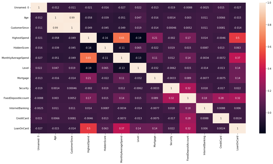
sns.heatmap(df.corr(), annot=True)
<AxesSubplot:>
Univariate analysis
import seaborn as sns
import matplotlib.pyplot as plt

#Number of data by Level
plt.figure(figsize=[10,5])
sns.countplot(x = 'Level',hue = 'LoanOnCard', data = df)
<AxesSubplot:xlabel='Level', ylabel='count'>
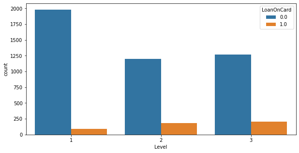
Observations:all values of level have different values; there is a variation
#Number of data by HiddenScore
plt.figure(figsize=[10,5])
sns.countplot(x = 'HiddenScore',hue = 'LoanOnCard', data = df)
<AxesSubplot:xlabel='HiddenScore', ylabel='count'>
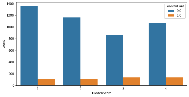
Observations:all values of HiddenScore have sufficient values; there is a variation
plt.figure(figsize=(20,5))
sns.countplot(x = 'Age', hue = 'LoanOnCard', data=df)
<AxesSubplot:xlabel='Age', ylabel='count'>

Observations: max age in between 30 - 60
#Pair plot
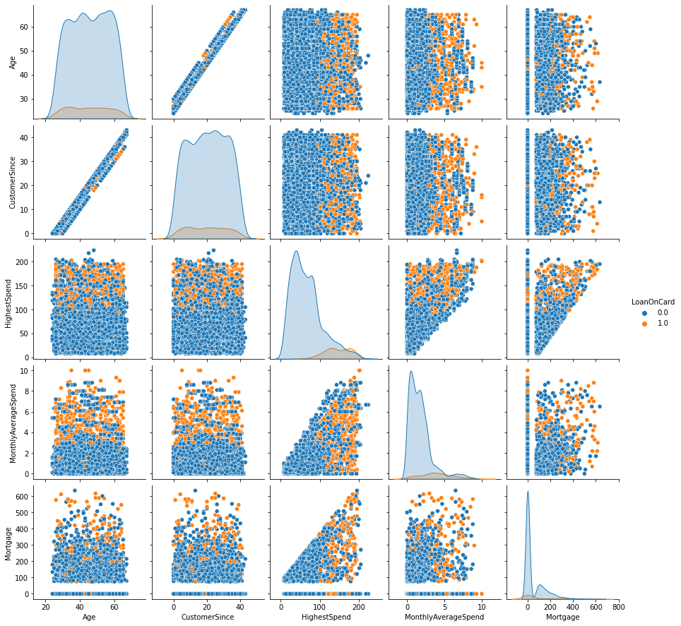
sns.pairplot(df, hue = 'LoanOnCard',
vars = ['Age', 'CustomerSince',
"HighestSpend","MonthlyAverageSpend","Mortgage"] )
<seaborn.axisgrid.PairGrid at 0x2132ea58>
plt.figure(figsize=(20,5))
sns.countplot(x = 'MonthlyAverageSpend', hue = 'LoanOnCard', data=df)
<AxesSubplot:xlabel='MonthlyAverageSpend', ylabel='count'>

plt.hist(df['MonthlyAverageSpend'])
(array([1670., 1346., 1017.,  319.,  218.,   97.,  131.,   80.,   45.,
           6.]),
 array([ 0.,  1.,  2.,  3.,  4.,  5.,  6.,  7.,  8.,  9., 10.]),
 <BarContainer object of 10 artists>)
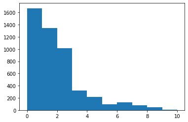
Observations: Most of the spend are within the range of 0 to 3
Preparing Data for Machine Learning Algorithms
#Let's drop the target coloumn before we do train test split
X = df.drop('LoanOnCard',axis=1)
y = df['LoanOnCard']
#Now we will split the data
from sklearn.model_selection import train_test_split
X_train, X_test, y_train, y_test = train_test_split(X, y, test_size=0.2, random_state=10)
Now we will split the data into training (80% of the data) and rest 20% - named test, will be kept aside for later use.
# Fitting Logistic Regression to the Training set
from sklearn.linear_model import LogisticRegression
classifier = LogisticRegression(random_state = 0)
classifier.fit(X_train, y_train)
C:\Users\ASUS\anaconda3\envs\py36\lib\site-packages\sklearn\linear_model\_logistic.py:765: ConvergenceWarning: lbfgs failed to converge (status=1):
STOP: TOTAL NO. of ITERATIONS REACHED LIMIT.

Increase the number of iterations (max_iter) or scale the data as shown in:
    https://scikit-learn.org/stable/modules/preprocessing.html
Please also refer to the documentation for alternative solver options:
    https://scikit-learn.org/stable/modules/linear_model.html#logistic-regression
  extra_warning_msg=_LOGISTIC_SOLVER_CONVERGENCE_MSG)
LogisticRegression(random_state=0)
Predicting the test data
#Predict
y_predict_test = classifier.predict(X_test)
Calculate the accuracy of the model
#Check accuracy
from sklearn.metrics import classification_report
print(classification_report(y_test, y_predict_test))
              precision    recall  f1-score   support

         0.0       0.95      0.98      0.97       880
         1.0       0.81      0.57      0.67       106

    accuracy                           0.94       986
   macro avg       0.88      0.78      0.82       986
weighted avg       0.93      0.94      0.93       986
Overall accuracy is pretty good (94%). Precision and recall for 1 is 81% and 57% respectively. We might hope to achieve a better result using a separate machine learning algorithm. In the next part we will use Decision Tree and try to improve the result.
Now we will be using Decision Tree
from sklearn.tree import DecisionTreeClassifier

classifier = DecisionTreeClassifier(random_state=0)
classifier.fit(X_train, y_train)
DecisionTreeClassifier(random_state=0)
Predict the test data
#Predict the model
y_pred = classifier.predict(X_test)
Calculate the accuracy of the model
#Check accuracy
from sklearn.metrics import classification_report
print(classification_report(y_test, y_pred))
              precision    recall  f1-score   support

         0.0       0.99      1.00      0.99       880
         1.0       0.99      0.92      0.95       106

    accuracy                           0.99       986
   macro avg       0.99      0.96      0.97       986
weighted avg       0.99      0.99      0.99       986
We can see that decision tree has improved the model significantly. Now I have both precision and recall above 90% with overall accuracy to be 99%